Finding the Governing Truck Position on a Bridge

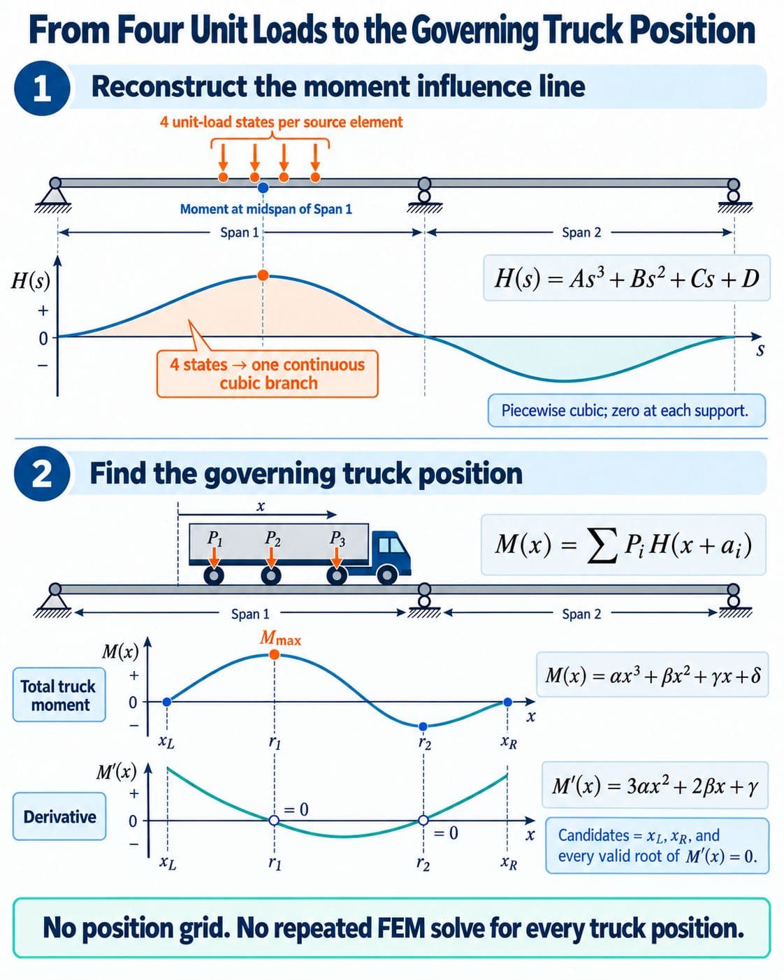
𝗛𝗼𝘄 𝗰𝗮𝗻 𝘄𝗲 𝗳𝗶𝗻𝗱 𝘁𝗵𝗲 𝗲𝘅𝗮𝗰𝘁 𝘁𝗿𝘂𝗰𝗸 𝗽𝗼𝘀𝗶𝘁𝗶𝗼𝗻 𝘁𝗵𝗮𝘁 𝗽𝗿𝗼𝗱𝘂𝗰𝗲𝘀 𝘁𝗵𝗲 𝗺𝗮𝘅𝗶𝗺𝘂𝗺 𝗯𝗲𝗻𝗱𝗶𝗻𝗴 𝗺𝗼𝗺𝗲𝗻𝘁 𝗼𝗻 𝗮 𝗯𝗿𝗶𝗱𝗴𝗲? 𝙎𝙩𝙚𝙥 1: 𝘽𝙪𝙞𝙡𝙙 𝙩𝙝𝙚 𝙢𝙤𝙢𝙚𝙣𝙩 𝙞𝙣𝙛𝙡𝙪𝙚𝙣𝙘𝙚 𝙡𝙞𝙣𝙚 • select one section of the bridge. • apply a unit load of 1 N at position s. • then calculate the bending moment at the selected section. A common method moves the unit load through many discrete positions. However: • Large spacing may miss a peak between two positions. • Small spacing requires many FEM solutions. 𝗛𝗲𝗿𝗲 𝗶𝘀 𝘁𝗵𝗲 𝗮𝗽𝗽𝗿𝗼𝗮𝗰𝗵 𝘂𝘀𝗲𝗱 𝗶𝗻 𝗼𝘂𝗿 𝗽𝗿𝗼𝗴𝗿𝗮𝗺. For a linear prismatic Euler–Bernoulli beam element, the moment influence response has the form: (this piecewise-cubic behavior comes from the cubic Hermite shape functions of the two-node Euler–Bernoulli beam element) H(s) = As³ + Bs² + Cs + D • We use four independent unit-load states for each source element. • These states give four moment values. The four values create four equations. The four equations determine A, B, C, and D. • We can then calculate H(s) at every position inside the branch. 𝗧𝗵𝗲 𝗿𝗲𝘀𝘂𝗹𝘁 𝗶𝘀 𝗮 𝗰𝗼𝗻𝘁𝗶𝗻𝘂𝗼𝘂𝘀 𝗰𝘂𝗯𝗶𝗰 𝗳𝘂𝗻𝗰𝘁𝗶𝗼𝗻. It is not only a collection of disconnected sample points. 𝙎𝙩𝙚𝙥 2: 𝙁𝙞𝙣𝙙 𝙩𝙝𝙚 𝙜𝙤𝙫𝙚𝙧𝙣𝙞𝙣𝙜 𝙩𝙧𝙪𝙘𝙠 𝙥𝙤𝙨𝙞𝙩𝙞𝙤𝙣 Let x represent the truck position. The total moment is: M(x) = Σ PᵢH(x + aᵢ) While every axle remains on its current influence-line branch, M(x) is also cubic: M(x) = αx³ + βx² + γx + δ The extreme value inside an interval may occur where: M′(x) = 0 The derivative is: M′(x) = 3αx² + 2βx + γ It may have zero, one, or two valid roots inside the interval. For every interval, the program checks: • The left endpoint. • The right endpoint. • Every derivative root inside the interval. Therefore, each interval has at most four candidate truck positions. The program evaluates all candidates. It then compares the candidates from every interval. The final result contains: • The maximum bending moment. • The governing truck position. • The position of every axle. • The contribution from each axle. 𝗡𝗼 𝗽𝗼𝘀𝗶𝘁𝗶𝗼𝗻 𝗴𝗿𝗶𝗱 𝗶𝘀 𝗿𝗲𝗾𝘂𝗶𝗿𝗲𝗱. 𝗡𝗼 𝗿𝗲𝗽𝗲𝗮𝘁𝗲𝗱 𝗙𝗘𝗠 𝘀𝗼𝗹𝘃𝗲 𝗶𝘀 𝗿𝗲𝗾𝘂𝗶𝗿𝗲𝗱 𝗳𝗼𝗿 𝗲𝘃𝗲𝗿𝘆 𝘁𝗿𝘂𝗰𝗸 𝗽𝗼𝘀𝗶𝘁𝗶𝗼𝗻. 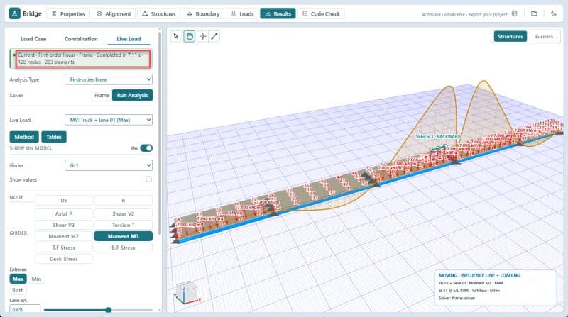𝗥𝗲𝗰𝗼𝗿𝗱𝗲𝗱 𝗿𝗲𝘀𝘂𝗹𝘁: In one recorded 20-lane benchmark with combined truck-and-lane loading, the complete Frame Solver pipeline completed about 7.0 seconds. We will share the Bridge tools when they are ready. Please stay tuned.